Fine-Tuning NVIDIA Cosmos Predict 2.5 with LoRA/DoRA for Robot Video Generation

Motivation

NVIDIA Cosmos Predict 2.5 is a large-scale world model capable of generating physically plausible videos conditioned on text, images, or video clips. To adapt it to a specific domain, such as robot manipulation or a particular camera viewpoint, teams still need targeted fine-tuning.

Training robot policies requires demonstration data, but collecting real-robot trajectories is slow and expensive. Generating synthetic trajectories with a fine-tuned video world model offers a scalable alternative. However, full fine-tuning of a 2B-parameter model is expensive and risks catastrophic forgetting of general knowledge. LoRA and DoRA inject small trainable adapter modules into the frozen base model, reducing memory requirements while keeping the adapter files small and portable. This makes it practical to fine-tune on a single GPU and flexibly swap adapters for different domains at inference.

This guide walks through parameter-efficient fine-tuning of Cosmos Predict 2.5 with LoRA and DoRA, using the diffusers and accelerate libraries with support for both single- and multi-GPU training. We then show how to use the fine-tuned model to generate synthetic robot trajectories for downstream robot learning tasks.

Requirements

• Python 3.10+
• PyTorch 2.5+ with CUDA
• diffusers (pulls in transformers and peft automatically), accelerate
• Optional: install wandb to monitor training
• At minimum one 80 GB GPU for single-GPU training; 8× H100s recommended for faster iteration

Install dependencies on your machine:

pip install -U "diffusers[torch]" transformers accelerate peft wandb 

---

Preparing Data

After installing diffusers, navigate to examples/cosmos to explore the example code.
We use the same datasets as the GR00T Dreams post-training recipe:

• Training Dataset: 92 robot manipulation videos with text prompts describing pick-and-place tasks.
• Test Dataset: 50 (prompt, image) pairs. The model should generate a video based on the input text prompt and the initial frame image.

Download and preprocess the training and test datasets using download_and_preprocess_datasets.sh:

bash download_and_preprocess_datasets.sh

The resulting training dataset folder looks like this:

gr1_dataset/train
├── metas/
│   └── *.txt
├── videos/
│   └── *.mp4
└── metadata.csv

The eval dataset is a flat directory of paired .txt and .png files for the (prompt, image) pairs:

gr1_dataset/test
├── filename1.txt
├── filename1.png
├── filename2.txt
├── filename2.png
└── ...

---

Training

In this section, we walk through the implementation in train_cosmos_predict25_lora.py.

VideoDataset

VideoDataset loads each sample as a (caption, video) pair from args.train_data_dir (gr1_dataset/train in our example). For videos longer than args.num_frames, it samples a random contiguous window of args.num_frames each epoch, enabling temporal augmentation. Internally, VideoProcessor from diffusers.video_processor resizes and normalizes the raw frames into a tensor of shape (channels, frames, height, width).

train_dataset = VideoDataset(
    dataset_dir=args.train_data_dir,
    num_frames=args.num_frames,
    video_size=[args.height, args.width],
)

Initialize Adapter

Cosmos Predict 2.5 consists of three submodules:

1. A VAE that encodes videos into latents
2. A text encoder that encodes text prompts into prompt embeddings
3. DiT for diffusion in the latent space

During training, all VAE, text encoder, and DiT weights are frozen. LoRA adapters are injected into the DiT's attention projections (to_q, to_k, to_v, to_out.0) and feedforward layers (ff.net.0.proj, ff.net.2). The trainable LoRA parameters are then upcast to float32 for numerical stability under bf16 mixed precision.

from diffusers import Cosmos2_5_PredictBasePipeline
from peft import LoraConfig

pipe = Cosmos2_5_PredictBasePipeline.from_pretrained(
    "nvidia/Cosmos-Predict2.5-2B",
    revision="diffusers/base/post-trained",
    torch_dtype=torch.bfloat16,
)

# freeze all base weights
dit = pipe.transformer
vae = pipe.vae
text_encoder = pipe.text_encoder

dit.requires_grad_(False)
vae.requires_grad_(False)
text_encoder.requires_grad_(False)

lora_config = LoraConfig(
    r=args.lora_rank,
    lora_alpha=args.lora_alpha,
    target_modules=['to_q', 'to_k', 'to_v', 'to_out.0', 'ff.net.0.proj', 'ff.net.2'],
    use_dora=args.use_dora,  # set True to switch to DoRA
)
dit.add_adapter(lora_config)
cast_training_params(dit, dtype=torch.float32)  # LoRA params in fp32

Passing use_dora=True switches to DoRA, which decomposes each weight into magnitude and direction before applying the low-rank update. No other changes to the training loop are needed.

Loss

Cosmos Predict 2.5 uses rectified flow: the model is trained to predict the velocity that linearly transports a noise sample toward the original "clean" data. Concretely, at timestep t, a noisy interpolation xt = σt·noise + (1−σt)·clean is constructed at a sampled noise level σt, and the model learns to predict the target velocity noise − clean via the mean-squared errors (MSE loss). The first two frames of the video are used as conditioning, and thus no noise is added to their latents..

The training loss follows the rectified flow formulation used by Cosmos Predict 2.5:

# Sample timestep with logit-normal distribution
sigma_t = sample_train_sigma_t(bsz, distribution='logitnormal', device=device)

# Rectified flow interpolates between clean latent and noise
xt = noise * sigma_t + clean_latent * (1 - sigma_t)

# Conditional generation: DiT conditions on the first two frames of the video, the timestep, and the prompt embeds
# `cond_indicator` and `cond_mask` have values = 1 for the first two frames and 0 for other frames
xt = clean_latent * cond_mask + xt * (1 - cond_mask)
in_timestep = cond_indicator * 0.0001 + (1 - cond_indicator) * sigma_t

# Forward
pred_velocity = dit(
                    hidden_states=xt,
                    condition_mask=cond_mask,
                    timestep=in_timestep,
                    encoder_hidden_states=prompt_embeds,
                    padding_mask=padding_mask,
                    return_dict=False,
                )[0]

# MSE loss is computed only on the non-conditioned frames
target_velocity = noise - clean_latent
pred_velocity = target_velocity * cond_mask + pred_velocity * (1 - cond_mask)
loss = F.mse_loss(pred_velocity.float(), target_velocity.float())

Optimizer and Scheduler

We use torch.optim.AdamW as the optimizer and get_linear_schedule_with_warmup from diffusers.optimization as the scheduler. The scheduler linearly warms up the learning rate over scheduler_warm_up_steps, peaks at scheduler_f_max × learning_rate, then linearly decays to scheduler_f_min × learning_rate over the remaining num_training_steps.

lora_params = [p for p in dit.parameters() if p.requires_grad]

optimizer = torch.optim.AdamW(lora_params, lr=args.learning_rate, weight_decay=args.weight_decay)
lr_scheduler = get_linear_schedule_with_warmup(
    optimizer,
    num_warmup_steps=args.scheduler_warm_up_steps,
    num_training_steps=args.num_training_steps,
    f_min=args.scheduler_f_min,
    f_max=args.scheduler_f_max,
)

Checkpointing

LoRA weights are saved in the diffusers format every args.checkpointing_epochs epochs:

if (epoch+1) % args.checkpointing_epochs == 0:
    if accelerator.is_main_process:
        save_path = os.path.join(args.output_dir, f"checkpoint-{epoch}")
        accelerator.save_state(save_path)

accelerator.save_state() writes a pytorch_lora_weights.safetensors file to save_path, which is the adapter file you will pass to the pipeline at inference time.

Training Command

Use the provided shell script as a starting point:

export MODEL_NAME="nvidia/Cosmos-Predict2.5-2B"
export DATA_DIR="gr1_dataset/train"
export OUT_DIR=YOUR_OUTPUT_DIR
lora_rank=32

accelerate launch --mixed_precision="bf16" train_cosmos_predict25_lora.py \
  --pretrained_model_name_or_path=$MODEL_NAME \
  --revision diffusers/base/post-trained \
  --train_data_dir=$DATA_DIR \
  --train_batch_size=1 \
  --num_train_epochs=500 \
  --checkpointing_epochs=100 \
  --seed=0 \
  --output_dir=$OUT_DIR \
  --report_to=wandb \
  --height 432 --width 768 \
  --allow_tf32 --gradient_checkpointing \
  --lora_rank $lora_rank --lora_alpha $lora_rank

lora_rank controls the rank of the low-rank decomposition. A higher rank means more trainable parameters and greater expressive capacity, at the cost of more memory and a larger adapter file. We use rank=32 as a starting point, resulting in ~50M trainable parameters.

lora_alpha is a scaling factor applied to the LoRA update: the weight delta is scaled by lora_alpha / lora_rank before being added to the frozen base weights. Setting lora_alpha = lora_rank (as done here) keeps this scale factor at 1.0, so the LoRA update is applied at full strength without any additional dampening.

To use DoRA instead of LoRA, add --use_dora to the command.

For multi-GPU training, accelerate handles the distribution automatically. Empirically, we find that training with 100 epochs already yields decent results on this task, which takes 17 hours on a single H100 and 2.5 hours on 8 H100 GPUs.

---

Running Inference with Your LoRA

Once training is complete, use eval_cosmos_predict25_lora.py to generate videos from the eval dataset. The script reads paired .png and .txt files from gr1_dataset/test, generates a video for each, and writes .mp4 files to --output_dir.

ImageDataset

ImageDataset reads the .txt file into a prompt string and uses load_image from diffusers.utils to load the .png as a PIL.Image.Image:

def __getitem__(self, idx):
    img_path, txt_path, stem = self.samples[idx]
    image = load_image(img_path)
    with open(txt_path) as f:
        prompt = f.read().strip()
    return {"image": image, "prompt": prompt, "stem": stem}

Loading the Pipeline and LoRA/DoRA Weights

from diffusers import Cosmos2_5_PredictBasePipeline

pipe = Cosmos2_5_PredictBasePipeline.from_pretrained(
    "nvidia/Cosmos-Predict2.5-2B",
    revision="diffusers/base/post-trained",
    device_map="cuda",
    torch_dtype=torch.bfloat16,
)

pipe.load_lora_weights("/path/to/lora/checkpoint")
pipe.fuse_lora(lora_scale=1.0)

fuse_lora merges the adapter weights into the base model, eliminating any inference overhead from the LoRA/DoRA decomposition.

Generating initial latent noise

To ensure reproducibility, the arch_invariant_rand function generates the initial latent noise via NumPy, making the noise invariant to GPU architectures. If reproducibility is not a concern, users do not need to provide input noise to the pipeline.

# generation starts from random noise with the same shape as the latent
latent_shape = pipe.get_latent_shape_cthw(args.height, args.width, args.num_output_frames)
noises = arch_invariant_rand(
    (args.batch_size, *latent_shape), dtype=torch.float32, device=args.device, seed=args.seed
)

frames = pipe(
    image=image,           # PIL Image: the conditioning first frame
    prompt=prompt,
    num_frames=args.num_output_frames,
    num_inference_steps=args.num_steps,
    height=args.height,
    width=args.width,
    latents=noises,        # optional
).frames[0]

export_to_video(frames, "output.mp4", fps=16)

Inference Command

export LORA_DIR=YOUR_ADAPTER_DIR
export DATA_DIR="gr1_dataset/test"
export OUT_DIR=YOUR_EVAL_OUTPUT_DIR

python eval_cosmos_predict25_lora.py \
  --data_dir $DATA_DIR \
  --output_dir $OUT_DIR \
  --lora_dir $LORA_DIR \
  --height 432 --width 768 \
  --num_output_frames 93 \
  --num_steps 36 \
  --seed 0

To evaluate the base model without any LoRA, omit --lora_dir.

---

Evaluation Metrics

Sampson Error

Sampson Error is a geometric error metric that measures the distance from matched keypoints to their corresponding epipolar lines. In the context of generated video, a low Sampson error means the motion between frames (or between camera views) is geometrically consistent. Higher values indicate jitter, hallucinated motion, or multi-view inconsistencies.

We follow the Cosmos Predict evaluation guide and evaluate the geometric quality of generated videos using two metrics:

• Temporal Sampson Error: computed between consecutive frames within a single camera view, measuring temporal stability.
• Cross-view Sampson Error: computed between simultaneous frames from different camera views, measuring multi-view geometric alignment.

LLM-as-a-Judge

We use Cosmos Reason2 as an LLM judge, scoring each example from 1 to 5. We design two rubrics:

• Physical plausibility (video_physics.yaml): the judge evaluates whether the video obeys physical commonsense, without seeing the text prompt.
• Instruction following (video_IF.yaml): the judge takes both the prompt and the video as input and evaluates whether the described task is completed correctly.

video_physics.yaml

system_prompt: "You are a helpful assistant."
user_prompt: |
  You are a helpful video analyzer. Evaluate whether the video follows physical commonsense.

  Evaluation Criteria:
  1. **Object Behavior:** Do objects behave according to their expected physical properties (e.g., rigid objects do not deform unnaturally, fluids flow naturally)?
  2. **Motion and Forces:** Are motions and forces depicted in the video consistent with real-world physics (e.g., gravity, inertia, conservation of momentum)?
  3. **Interactions:** Do objects interact with each other and their environment in a plausible manner (e.g., no unnatural penetration, appropriate reactions on impact)?
  4. **Consistency Over Time:** Does the video maintain consistency across frames without abrupt, unexplainable changes in object behavior or motion?

  Instructions for Scoring:
  - **1:** No adherence to physical commonsense. The video contains numerous violations of fundamental physical laws.
  - **2:** Poor adherence. Some elements follow physics, but major violations are present.
  - **3:** Moderate adherence. The video follows physics for the most part but contains noticeable inconsistencies.
  - **4:** Good adherence. Most elements in the video follow physical laws, with only minor issues.
  - **5:** Perfect adherence. The video demonstrates a strong understanding of physical commonsense with no violations.

  Does this video adhere to the physical laws?

video_IF.yaml

system_prompt: "You are a helpful assistant."
user_prompt: |
  You are a helpful video analyzer. Evaluate whether the video follows the given instruction.

  Instruction: {instruction}

  Evaluation Criteria:
  1. **Task Completion:** Does the video show the task described in the instruction being completed?
  2. **Action Accuracy:** Are the actions performed in the video consistent with what the instruction specifies?
  3. **Object Interaction:** Does the robot or agent interact with the correct objects as described in the instruction?
  4. **Goal Achievement:** Is the final state of the video consistent with the expected outcome of the instruction?
  5. **Correct Hand Usage:** Does the video show the correct hand performing the action?

  Instructions for Scoring:
  - **1:** No adherence to the instruction. The video shows actions completely unrelated to the instruction.
  - **2:** Poor adherence. Some elements match the instruction, but major deviations are present.
  - **3:** Moderate adherence. The video follows the instruction for the most part but contains noticeable deviations.
  - **4:** Good adherence. Most elements in the video match the instruction, with only minor issues.
  - **5:** Perfect adherence. The video fully follows the instruction with no deviations.

  Does this video follow the instruction?

Results

Qualitative Analysis

We compare videos generated by the base model (before fine-tuning), LoRA, and DoRA on the first two examples from the test set.

Prompt: Use the left hand to pick up dark green cucumber from on circular gray mat to above beige bowl.

Before Training	LoRA r=32	DoRA r=32

Prompt: Use the right hand to pick up orange juice carton from center of pink plate to center of green bowl.

Before Training	LoRA r=32	DoRA r=32

Before fine-tuning, the base model struggles in several ways: robot hands are out-of-distribution, causing the model to hallucinate human hands in later frames; it does not reliably use the correct hand specified in the prompt; and the generated videos exhibit noticeable jitter. Fine-tuning with LoRA and DoRA addresses all three issues.

Quantitative Analysis

We fine-tune four adapters under different settings: LoRA and DoRA with rank 8 and 32. For each test example, we generate 5 videos with different seeds and report the average score across seeds, using the three metrics introduced in the Evaluation Metrics section.

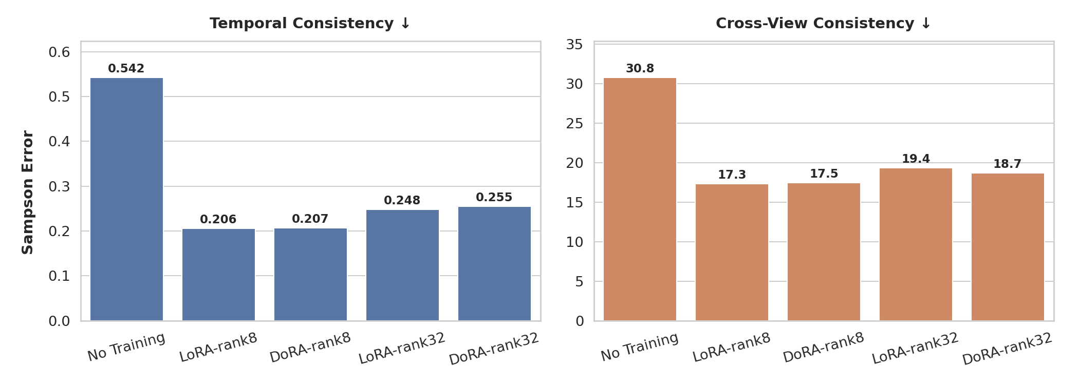
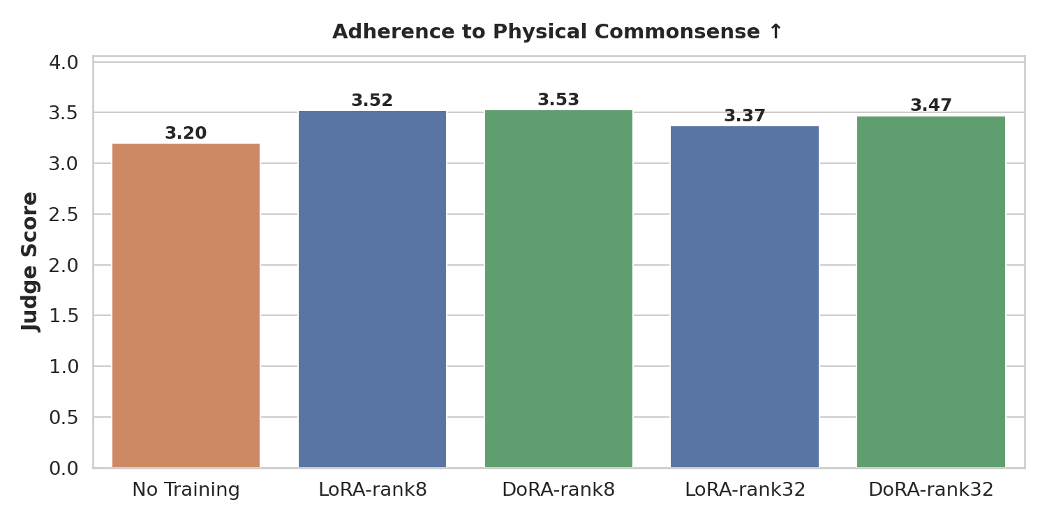
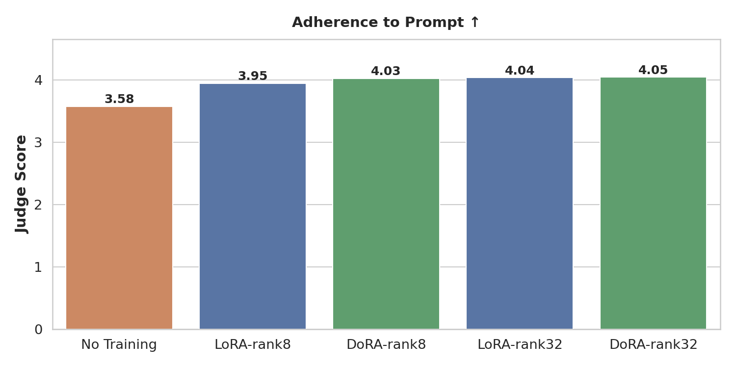
Conclusion: Training for 100 epochs (~2.5 hours on 8× H100s) is already sufficient to substantially improve all three metrics. Both LoRA and DoRA converge to similar performance, confirming that the extra magnitude-direction decomposition in DoRA does not hurt and may help at very low ranks, but is not necessary here.

Larger rank (32 vs 8) boosts instruction following (the model has more capacity to learn precisely which hand to use and which objects to interact with), but does not improve geometric consistency or physical plausibility. We hypothesize that this is because geometric and physical priors are largely captured by the world model's frozen weights; the LoRA adapter only needs to shift the distribution toward in-domain robot appearance and task structure, which is achievable at rank 8.

When to use DoRA vs LoRA: If memory is very tight or adapter file size matters, start with LoRA r=8. If you have budgets and observe training instability with LoRA at low rank, DoRA r=32 is a reasonable alternative, as the magnitude–direction decomposition can help stabilize learning.

• Visit our Cosmos Cookbook for step-by-step workflows, technical recipes, and concrete examples for building, adapting, and deploying Cosmos WFMs.
• Explore new open Cosmos models and datasets on Hugging Face and GitHub or try models on build.nvidia.com.
• Be part of the community and join our Cosmos Discord channel.
• Already using Cosmos? Learn more about how to contribute.

Upvote

-

Models mentioned in this article 1

Datasets mentioned in this article 1